4.5. Lecture 11#
Error propagation: functions of uncertain parameters#
To propagate errors, we need to know the answer to: Given a posterior for \(X\), what is the posterior for \(Y = f(X)\)?
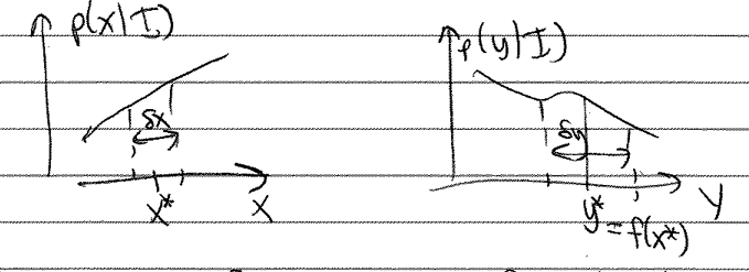
Here is a schematic of the posteriors for \(X\) and \(Y\) (the notation is that \(x\) is an instance of the random variable denoted \(X\)):

We are assuming here that there is a 1-1 mapping of the function.
So what do we know? The probability in the interval shown in each picture must be the same, regardless of what variable is used, \(X\) or \(Y\). Note that this is the probability, not the probability density. Therefore
This must be true for all \(x^*\), so in the \(\delta x,\delta y \rightarrow 0\) limit we must have
An alternative derivation uses marginalization and the fact that \(y = f(x)\) means the pdf \(p(y|x,I)\) is a delta function:
where we have used the properties of delta functions. So it is really just a matter of changing variables.
As an example of how a more naive (but apparently faster) approach can fail badly, consider the example from Sivia 3.6.2 in the notebook: Example: Propagation of systematic errors
Visualization of the Central Limit Theorem (CLT)#
Go through the Visualization of the Central Limit Theorem notebook.
Follow-up to CLT proof for Poisson distribution#
In an assignment you proved that in the limit \(D \rightarrow \infty\)
using Stirling’s formula: \(x! \rightarrow \sqrt{2\pi x}e^{-x} x^x\) as \(x\rightarrow\infty\) and letting \(x = N = D(1+\delta)\) where \(D\gg 1\) and \(\delta \ll 1\), plus \((1+\delta)^a = e^{a\ln (1+\delta)}\).
In carrying out this proof, the term \(D\delta^2/2\) is kept but \(\delta/2\) is dropped. Why?
Because \(N-D\) is of order the standard deviation of the distribution, which is \(\sqrt{D}\). But \(N-D = D\delta\), so \(D\delta \sim \sqrt{D} \gg 1\), which means \(D\delta^2/2 = \delta/2 (D\delta) \gg \delta/2\).
PDF Manipulations I: Combining random variables#
Adding independent random variables#
Suppose we have two random variables, \(X\) and \(Y\), drawn from two different distributions.
For concreteness we’ll take the distributions to be Gaussian (normal) with different means and widths, and independent of each other.
\[\begin{split}\begin{align} X | \mu_x,\sigma_x &\sim \mathcal{N}(\mu_x,\sigma_x^2) \quad\Longleftrightarrow\quad p(x|\mu_x,\sigma_x) = \frac{1}{\sqrt{2\pi}\sigma_x}e^{-(x-\mu_x)^2/2\sigma_x^2} \\ Y | \mu_y,\sigma_y &\sim \mathcal{N}(\mu_y,\sigma_y^2) \quad\Longleftrightarrow\quad p(y|\mu_y,\sigma_y) = \frac{1}{\sqrt{2\pi}\sigma_y}e^{-(y-\mu_y)^2/2\sigma_y^2} \end{align}\end{split}\]What is the distribution of the sum of \(X\) and \(Y\)?
From past experience, we might expect that “errors add in quadrature”, but how does that arise in detail?
This is a special case of uncertainty propagation: How do errors combine?
First phrase the question in terms of a statement about posteriors
Goal: given \(Z=X+Y\), how is \(Z\) distributed, i.e., what is \(p(z|I)\)?
Plan: follow the same steps as with the CLT proof! (We’ll suppress the explicit information \(I\)’s here for conciseness.)
(4.2)#\[\begin{split}\begin{align} p(z) &= \int_{-\infty}^{\infty} dx\,dy\, p(z,x,y) \\ &= \int_{-\infty}^{\infty} dx\,dy\, p(z|x,y) p(x,y) \\ &= \int_{-\infty}^{\infty} dx\,dy\, p(z|x,y) p(x) p(y) \end{align}\end{split}\]What is the justification for each of the three steps?
Marginalization, product rule, independence. What if \(X\) and \(Y\) are not independent?
What is \(p(z|x,y)\)?
(4.3)#\[ p(z|x,y) = \delta(z-x-y) = \frac{1}{2\pi} \int_{-\infty}^{\infty} d\omega\, e^{-i\omega\left(z-(x+y)\right)} = \frac{1}{2\pi} \int_{-\infty}^{\infty} d\omega\, e^{-i\omega z} e^{i\omega x} e^{i\omega y} \]We choose the Fourier representation of the delta function because the dependence on \(x\) and \(y\) factorizes. That is, the dependence appears as a product of a function of \(x\) times a function of \(y\). (But we don’t need to do that for Gaussians; we can just use the delta function to do one integral and evaluate the second one directly.)
Now we can substitute the result for \(p(z|x,y)\) into the final expression for \(p(z)\) and observe that the integrals factorize. Note: at this stage we have used independence of \(X\) and \(Y\) but we haven’t used that they are Gaussian distributed. So we get:
(4.4)#\[\begin{split}\begin{align} p(z) &= \int_{-\infty}^{\infty} dx \int_{-\infty}^{\infty} dy \left(\int_{-\infty}^{\infty} \frac{d\omega}{2\pi} e^{-i\omega z}\right) e^{i\omega x} p(x)\, e^{i\omega y} p(y) \\ &= \int_{-\infty}^{\infty} \frac{d\omega}{2\pi} e^{-i\omega z} \left[\int_{-\infty}^{\infty} dx\, e^{i\omega x}p(x)\right] \left[\int_{-\infty}^{\infty} dy\, e^{i\omega y}p(y)\right] \end{align}\end{split}\][Note: we really should verify that the functions are such that we can change integration orders to get the last line!]
We now need the Fourier transforms of the pdfs for \(X\) and \(Y\). Finally we’ll get specific and use Gaussians:
(4.5)#\[\begin{split}\begin{align} \int_{-\infty}^{\infty} dx\, e^{i\omega x} \frac{1}{\sqrt{2\pi}\sigma_x}e^{-(x-\mu_x)^2/2\sigma_x^2} & = e^{i\mu_x\omega}e^{-\sigma_x^2\omega^2/2} \\ \int_{-\infty}^{\infty} dy\, e^{i\omega y} \frac{1}{\sqrt{2\pi}\sigma_y}e^{-(y-\mu_y)^2/2\sigma_y^2} & = e^{i\mu_y\omega}e^{-\sigma_y^2\omega^2/2} \\ \end{align}\end{split}\]Here we have used \(\int_{-\infty}^{\infty} e^{\pm iax} e^{-bx^2}dx = \sqrt{\frac{\pi}{b}} e^{-a^2/4b}\).
Next substitute the FT’s into the expression for \(p(z)\):
(4.6)#\[\begin{split}\begin{align} p(z) &= \int_{-\infty}^{\infty} \frac{d\omega}{2\pi} e^{-i\omega (z - \mu_x - \mu_y)} e^{-\omega^2(\sigma_x^2 + \sigma_y^2)/2} \\ &= \frac{1}{2\pi} \sqrt{\frac{2\pi}{\sigma_x^2 + \sigma_y^2}} e^{-(z - (\mu_x + \mu_y))^2/2(\sigma_x^2 + \sigma_y^2)} \\ &= \frac{1}{\sqrt{2\pi}\sqrt{\sigma_x^2 + \sigma_y^2}} e^{-(z - (\mu_x + \mu_y))^2/2(\sigma_x^2 + \sigma_y^2)} \end{align}\end{split}\]Thus: \(X+Y \sim \mathcal{N}(\mu_x+\mu_y, \sigma_x^2 + \sigma_y^2)\) or the means add and the variances add (not the standard deviations).
Generalizations:
\(X-Y\) \(\Lra\) Now \(p(z|x,y) = \delta(z-(x-y))\) and the minus sign here takes \(e^{i\omega y} \rightarrow e^{-i\omega y}\) and the FT yields \(e^{-i\mu_y\omega}\) \(\Lra\) \(\mathcal{N}(\mu_x - \mu_y, \sigma_x^2 + \sigma_y^2)\).
\(aX + bY\) for any \(a,b\) \(\Lra\) Now \(p(z|x,y) = \delta(z-(ax+by))\) which yields \(e^{-i\omega z}e^{ia\omega x}e^{ib\omega y}\). We show an example of how this means \(\mu_x \rightarrow a\mu_x\) and \(\sigma_x^2 \rightarrow a^2\sigma_x^2\) and similarly with \(b\), leading to
\[\begin{split}\begin{align} \int_{-\infty}^{\infty}dx\, e^{ia\omega x} \frac{1}{\sqrt{2\pi}\sigma_x}e^{-(x-\mu_x)^2/2\sigma_x^2} &= e^{ia\mu_x\omega}e^{-a^2\sigma_x^2\omega^2} \\ &\Lra aX + bY \sim \mathcal{N}(a\mu_x+b\mu_y, a^2\sigma_x^2+b^2\sigma_y^2) . \end{align}\end{split}\]Note that this last example includes \(X\pm Y\) as special cases.
Finally, we can sum \(m\) Gaussian random variables, following all the same steps, to find
\[ X_1 + X_2 + \cdots + X_m \sim \mathcal{N}(\mu_1 + \mu_2 + \cdots+\mu_m, \sigma_1^2 + \sigma_2^2 + \cdots + \sigma_m^2) . \]
Last generalization: adding multivariate normals#
Now suppose \(X\) and \(Y\) are themselves random variables from (independent) multivariate normal distributions of dimension \(N\) while \(A,B\) are known \(M\times N\) matrices. So
\[ X \sim \mathcal{N}(\muvec_x, \Sigmavec_x), \qquad Y \sim \mathcal{N}(\muvec_y, \Sigmavec_y), \]where \(\muvec_x, \muvec_y\) are \(N\)-dimensional vectors and \(\Sigmavec_x,\Sigmavec_y\) are \(N\times N\) covariance matrices.
The claim is that:
\[ A X + B Y \sim \mathcal{N}(A\muvec_x + B\muvec_y, A\Sigmavec_x A^\intercal + B\Sigmavec_y B^\intercal) . \]
Check that the matrix-vector multiplications work
\(A\muvec_x \Lra (M\times N)\cdot N\) gives \(M\) correctly; \(A\Sigmavec_x A^\intercal \Lra (M\times N)\cdot(N\times N)\cdot(N\times M)\) gives \(M\times M\) correctly.
If we apply this for \(A \rightarrow a I_N\) and \(B \rightarrow b I_N\), where \(a,b\) are scalars and \(I_N\) is the \(N\times N\) identity, then it is much simpler:
\[ a X + b Y \sim \mathcal{N}(a\muvec_x + b\muvec_y, a^2\Sigmavec_x + b^2 \Sigmavec_y). \]So the covariance matrices add in quadrature!
