Lecture 4: A couple of frequentist connections

1.10. Lecture 4: A couple of frequentist connections#

The near ubiquity of Gaussians#

In the last lecture we considered a Gaussian distribution and estimated its mean and variance. We are going to see a lot of Gaussian distributions in this course. And indeed some people implicitly always assume Gaussian distributions. So this seems like as good a place as any to pause and consider why Gaussian distributions are a common choice to describe noise, as well as thinking about the circumstances in which that choice might be a poor one.

It turns out there are several reasons why one might choose a Gaussian to describe a probability distribution. Here are two:

The Gaussian is to statistics what the harmonic oscillator is to mechanics#

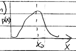
Suppose we have a probability distribution \(p(x | D,I)\) that is unimodal (has only one hump), then one way to form a “best estimate’’ for the variable \(x\) is to compute the maximum of the distribution. (To save writing we denote the pdf of interest as \(p(x)\) for a while hereafter.)

We find this point, which we’ll denote by \(x_0\), using calculus:

\[ \left.\frac{dp}{dx}\right|_{x_0} = 0 \quad \mbox{with} \quad \left.\frac{d^2p}{dx^2}\right|_{x_0} < 0 \ \text{(maximum)}. \]

To characterize the posterior \(p(x)\), we look nearby. We want to know how sharp this maximum is: is \(p(x)\) sharply peaked around \(x=x_0\) or is the maximum kind-of shallow? To work this out we’ll do a Taylor expansion around \(x=x_0\). \(p(x)\) itself varies too fast, but since \(p(x)\) is positive definite we can Taylor expand \(\log p\) instead. (See the box below for a strict mathematical reason why it’s a bad idea to directly Taylor expand \(p(x)\) around its maximum.)

\[ \Longrightarrow\ L(x) \equiv \log p(x|D,I) = L(x_0) + \left.\frac{dL}{dx}\right|_{x_0 = 0} + \frac{1}{2} \left.\frac{d^2L}{dx^2}\right|_{x_0 = 0}(x-x_0)^2 + \cdots \]

Note that \(\left.\frac{dL}{dx}\right|_{x_0 = 0}=0\) (\(L(x_0)\) is also a maximum) and \(\left.\frac{d^2L}{dx^2}\right|_{x_0 = 0} < 0\). If we can neglect higher-order terms, then when we re-exponentiate,

\[ p(x| D,I) \approx A\, e^{\frac{1}{2}\left.\frac{d^2L}{dx^2}\right|_{x_0 = 0}(x-x_0)^2} , \]

with \(A\) a normalization factor. So in this general circumstance we get a Gaussian. Comparing to

\[ p(x|D,I) = \frac{1}{\sqrt{2\pi\sigma^2}}e^{-(x-\mu)^2/\sigma^2} \quad\Longrightarrow\quad \mu = x_0, \ \sigma = \left(-\left.\frac{d^2L}{dx^2}\right|_{x_0}\right)^{-1/2}, \]

where we see the importance of the second derivative being negative.

We usually quote \(x = x_0 \pm \sigma\), because if it is a Gaussian this is sufficient to tell us the entire distribution and \(n\) standard deviations is \(n\times \sigma\).
But for a Bayesian, the full posterior \(p(x|D,I)\) for all \(x\) is the general result, and \(x = x_0 \pm \sigma\) may be only an approximate characterization.

To think about …

What if \(p(x|D,I)\) is asymmetric? What if it is multimodal?

\(p\) or \(\log p\)?

We motivated Gaussian approximations from a Taylor expansion to quadratic order of the logarithm of a pdf. What would go wrong if we directly expanded the pdf? Well, if we do that we get:

\[ p(x) \approx p(x_0) + \frac{1}{2}\left.\frac{d^2p}{dx^2}\right|_{x_0}(x-x_0)^2 \ \overset{x\pm\rightarrow\infty}{\longrightarrow} -\infty, \]

i.e., we get something that diverges as \(x\) tends to either plus or minus infinity.

A pdf must be normalizable and positive definite, so this approximation violates these conditions!

The Central Limit Theorem#

Another reason a Gaussian pdf emerges in many calculations is because the Central Limit Theorem (CLT) states that the sum of random variables drawn from all (or almost all) probability distributions will eventually produce Gaussians if the number of samples in each sum is large enough.

Central Limit Theorem: The sum of \(n\) random values drawn from any pdf of finite variance \(\sigma^2\) tends as \(n \rightarrow \infty\) to be Gaussian distributed about the expectation value of the sum, with variance \(n \sigma^2\).

Consequences:#

The mean of a large number of values becomes normally distributed regardless of the probability distribution the values are drawn from.
The binomial, Poisson, chi-squared, and Student’s t- distributions all approach Gaussian distributions in the limit of a large number of degrees of freedom (e.q., for large \(n\) for binomial). This consequence is probably not immediately obvious to you from the statement of the CLT! (See the Visualization of the Central Limit Theorem notebook for an explanation of the Poisson distribution.)

Question

Why would we expect the CLT to work for a binomial distribution?

Hint

If we denote Bin(\(n,p\)) as the binomial distribution for \(n\) trials with probability \(p\) of success, how is Bin(\(1,p\)) related to Bin(\(n,p\))?

Answer

If we add up \(n\) random variables from Bin(\(1,p\)), each with value 0 or 1, this is equivalent to a Bin(\(n,p\)) random variable with the same number of successes. So we already have a sum of random variables built in and the CLT will apply. (In more detail: getting \(k\) ones (and \(n-k\) zeros) from the \(n\) Bin(\(1,p\)) draws will have probability \(p^k\) times \((1-p)^{n-k}\) times the number of combinations \(n\choose k\). This is the same as the binomial probability for \(k\) successes.)

Proof of the CLT in a special case:#

Start with independent random variables \(x_1,\cdots,x_n\) drawn from a distribution with mean \(\langle x \rangle = 0\) and variance \(\langle x^2\rangle = \sigma^2\), where

\[ \langle x^n \rangle \equiv \int x^n p(x)\, dx \]

(generalize later to nonzero mean). Now let

\[ X = \frac{1}{\sqrt{n}}(x_1 + x_2 + \cdots + x_n) = \sum_{j=1}^n \frac{x_j}{\sqrt{n}} , \]

(we scale by \(1/\sqrt{n}\) so that \(X\) is finite in the \(n\rightarrow\infty\) limit).

What is the distribution of \(X\)? \(\Longrightarrow\) call it \(p(X|I)\), where \(I\) is the information about the probability distribution for \(x_j\).

Plan: Use the sum and product rules and their consequences to relate \(p(X)\) to what we know of \(p(x_j)\). (Note: we’ll suppress \(I\) to keep the formulas from getting too cluttered.)

\[\begin{split}\begin{align} p(X) &= \int_{-\infty}^{\infty} dx_1 \cdots dx_n\, p(X,x_1,\cdots,x_n) \\ &= \int_{-\infty}^{\infty} dx_1 \cdots dx_n\, p(X|x_1,\cdots,x_n)\,p(x_1,\cdots,x_n) \\ &= \int_{-\infty}^{\infty} dx_1 \cdots dx_n\, p(X|x_1,\cdots,x_n)\,p(x_1)\cdots p(x_n) . \end{align}\end{split}\]

Class: state the rule used to justify each step

marginalization
product rule
independence

We might proceed by using a direct, normalized expression for \(p(X|x_1,\cdots,x_n)\):

Question

What is \(p(X|x_1,\cdots,x_n)\)?

Answer

\(p(X|x_1,\cdots,x_n) = \delta\Bigl(X - \frac{1}{\sqrt{n}}(x_1 + \cdots + x_n)\Bigr)\)

Instead we will use a Fourier representation:

\[ p(X|x_1,\cdots,x_n) = \delta\Bigl(X - \frac{1}{\sqrt{n}}(x_1 + \cdots + x_n)\Bigr) = \frac{1}{2\pi} \int_{-\infty}^{\infty} d\omega \, e^{i\omega\Bigl(X - \frac{1}{\sqrt{n}}\sum_{j=1}^n x_j\Bigr)} . \]

Substituting into \(p(X)\) and gathering together all pieces with \(x_j\) dependence while exchanging the order of integrations:

\[ p(X) = \frac{1}{2\pi} \int_{-\infty}^{\infty} d\omega \, e^{i\omega X} \prod_{j=1}^n \left[\int_{-\infty}^{\infty} dx_j\, e^{i\omega x_j / \sqrt{n}} p(x_j) \right] \]

Observe that the terms in []s have factorized into a product of independent integrals and they are all the same (just different labels for the integration variables).
Now we Taylor expand \(e^{i\omega x_j/\sqrt{n}}\), arguing that the Fourier integral is dominated by small \(x\) as \(n\rightarrow\infty\). (When does this fail?)

\[ e^{i\omega x/\sqrt{n}} = 1 + \frac{i\omega x}{\sqrt{n}} + \frac{(i\omega)^2 x^2}{2 n} + \mathcal{O}\left(\frac{\omega^3 x^3}{n^{3/2}}\right) \]

Then, using that \(p(x)\) is normalized (i.e., \(\int_{-\infty}^{\infty} dx\, p(x) = 1\)),

\[\begin{split} \begin{align} \int_{-\infty}^{\infty} dx\, e^{i\omega x / \sqrt{n}} p(x)&= \int_{-\infty}^\infty dx p(x) \left[1 +\frac{ i \omega x}{\sqrt{n}} + \frac{(i \omega)^2 x^2}{2 n} + \ldots\right]\\ &=1 + \frac{i \omega}{\sqrt{n}} \langle x \rangle - \frac{\omega^2}{2 n} \langle x^2 \rangle + \langle x^3 \rangle \frac{\omega^3}{n^{3/2}}\\ &=1 - \frac{\omega^2 \sigma^2}{2 n} + \mathcal{O}\left(\frac{\omega^3}{n^{3/2}}\right) \end{align} \end{split}\]

Now we can substitute into the posterior for \(X\) and take the large \(n\) limit:

\[\begin{split} \begin{align} p(X)&=\frac{1}{2 \pi} \int_{-\infty}^\infty d \omega e^{i \omega X} \left[1 - \frac{\omega^2 \sigma^2}{2 n} + \mathcal{O} \left(\frac{\omega^3}{n^{3/2}}\right)\right]^n\\ &\stackrel{n\rightarrow \infty}{\longrightarrow} \frac{1}{2 \pi} \int d\omega e^{i \omega X} e^{- \omega^2 \sigma^2/2}=\frac{1}{\sqrt{2 \pi}} e^{-X^2/(2 \sigma^2)}. \end{align} \end{split}\]

Notebook:#

Look at Visualization of the Central Limit Theorem.

Things to think about:

What does ``large’’ number of degrees of freedom actually mean? Does it matter where we look?
If we have a large number of draws from a uniform distribution, does the CLT imply that the histogrammed distribution should look like a Gaussian?
Can you identify a case where the CLT will fail?

p-values: when all you can do is falsify#

A common way for a frequentist to discuss a theory/model, or put a bound on a parameter value, is to quote a p-value.
This is set up using something called the null hypothesis. Somewhat perversely you should pick the null hypothesis to be the opposite of what you want to prove. So if you want to discover the Higgs boson, the null hypothesis is that the Higgs boson does not exist.
Then you pick a level of proof you are comfortable with. For the Higgs boson (and for many other particle physics experiments) it is “5 sigma’’. How do you think we convert this statement to a probability?
One minus the resulting probability is called the \(p\)-value. We will denote it \(p_{\rm crit}\). There is nothing God-given about it. It is a standard (like “beyond a reasonable doubt”) that has been agreed upon in a research community for determining that something is (likely) going on.
You then take data and compute \(p(D|{\rm null~hypothesis})\). If \(p(D|{\rm null~ hypothesis}) < p_{\rm crit}\) then you conclude that the “the null hypothesis is rejected at the \(p_{\rm crit}\) significance level’’.
Note that if \(p(D|{\rm null~hypothesis}) > p_{\rm crit}\) you cannot conclude that the null hypothesis is true. It just means “no effect was observed”.

Exercise

Look at Interactive Bayesian updating: coin flipping example. Pick a \(p_{\rm crit}\)-value. If \(p_h=0.4\), work out how many coin tosses it would take to reject the null hypothesis that it’s a fair coin (\(p_h=0.5\)) at this significance level.

Contrast Bayesian and significance analyses for coin flipping#

Suppose we do a coin flipping experiment where we toss a coin 20 times and it comes up heads 14 times. Let’s compare how we might analyze this with Bayesian methods to how we might do a significance analysis with p-values.

Bayesian analysis. Following our study in Interactive Bayesian updating: coin flipping example, let’s calculate the probability of heads, which we call \(p_h\), given data \(D = \{R \text{ heads}, N \text{ tosses}\}\).

Let’s assume a uniform prior (encoded as a beta function with \(\alpha=1\), \(\beta=1\)).
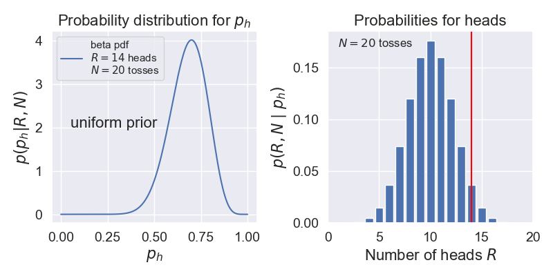
We found that this can be expressed as a beta function, which we can calculate in Python using \(p(p_h|D) = p(D|p_h)p(p_h)\) \(\longrightarrow\) scipy.stats.beta.pdf(p_h,1+R,1+N-R). For \(N=20\), \(R=14\), this is shown on the left below.
Now we can answer many questions, such as: what is the probability that \(p_h\) is between \(0.49\) and \(0.51\)? The answer comes from integrating our pdf over this interval (i.e., the area under the curve).
Note that in the Bayesian analysis, the data is given while the probability of heads is a random value.

Significance test. Here we will try to answer the question: Is the coin fair? We’ll follow the discussion in Wikipedia under p-value titled “Testing the fairness of a coin”.

We interpret “fair” as meaning \(p_h = 0.5\). Our null hypothesis is that the coin is fair and \(p_h = 0.5\).
We plot the probabilities for getting \(R\) heads in \(N=20\) tosses using the binomial probability mass distribution on the right above.
We decide on the significance \(p_{\rm crit} = 0.05\).
(Important conceptual question:) \(p_{\rm crit}\) and \(p_h\) are both probabilities. Turn to your neighbor and explain to them what they are the probabilities of and how they are different.
We need to find the probability of getting data at least as extreme as \(D = \{R \text{ heads}, N \text{ tosses}\}\). For our example, that means adding up the binomial probabilities for \(R = 14, 15, \ldots, 20\), which is 0.058. (This is called a “one-tailed test”. If we wanted to consider deviations favoring tails as well, we would would add as well the probabilities for \(R = 0, 1, \ldots, 6\), so \(0.115\) in total. This would be a “two-tailed test”.)
Comparing to \(p_{\rm crit} = 0.05\), we find the p-value is greater than \(p_{\rm crit}\), so the null hypothesis is not rejected at the 95% level. (Note that we say “not rejected” as opposed to “accepted”.) If we had gotten 15 heads instead we would have rejected the null hypothesis.
Note that in this frequentist analysis, the data is random while \(p_h\) is fixed (although unknown).

Exercise

Verify that if we had gotten 15 heads in \(N=20\) tosses that we would have rejected the null hypothesis.

Bayesian degree of belief intervals and frequentist confidence intervals#

In class on Wednesday we also talked about the difference between the 68% degree of belief interval for the most likely value (in that case the bias weighting of the coin) and a frequentist \(1 \sigma\) confidence interval.

First point is that \(1 \sigma=68\)% assumes a Gaussian distribution around the maximum of the posterior (cf. above). While this will often work out okay, it may not. And, as we seek to translate, \(n \sigma\) intervals into DoB statements, assuming a Gaussian becomes more and more questionable the higher \(n\) is. (Why?)
But the second point is more philosophical (meta-statistical?). One interval is a statement about \(p(x|D,I)\), while the other is a statement about \(p(D|x,I)\).
(Note that because the conversion between the two pdfs requires the use of Bayes’ theorem the Bayesian interval may be affected by the choice of the prior.)
Bayesian version is easy; a 68% credible interval or Bayesian confidence interval or degree-of-belief (DoB) interval is: given some data and some information \(I\), there is a 68% chance (probability) that the interval contains the true parameter.
Frequentist 68% confidence interval
- Assuming the model (contained in \(I\)) and the value of the parameter \(x\) then if we do the experiment a large number of times then 68% of them will produce data in that interval.
- So the parameter is fixed (no pdf) and the confidence interval is a statement about data
- Frequentists will try to make statements about parameters, but they end up a bit tangled, e.g., “There is a 68% probability that when I compute a confidence interval from data of this sort that the true value of \(\theta\) will fall within the (hypothetical) space of observations.”
For a one-dimensional posterior that is symmetric, it is clear how to define the \(d\%\) confidence interval.
- Algorithm: start from the center, step outward on both sides, stop when \(d\%\) is enclosed.
- For a two-dimensional posterior, need a way to integrate from the top. (Could lower a plane, as desribed below for HPD.)
What if asymmetic or multimodal? Two of the possible choices:
- Equal-tailed interval (central interval): the area above and below the interval are equal.
- Highest posterior density (HPD) region: posterior density for every point is higher than the posterior density for any point outside the interval. [E.g., lower a horizontal line over the distribution until the desired interval percentage is covered by regions above the line.]