Lecture 2

1.4. Lecture 2#

Follow-ups to Lecture 1 notebooks#

Notes on filling in the table in Checking the sum and product rules, and their consequences using Python:
- fstring: print(f'ratio = {ratio:.3f}') or np.around(number,digits)
- How do you use numpy arrays?
- experts: write function to work with either ints or floats or numpy arrays
Further takeaways from Exploring PDFs to discuss in class
- Bayesian confidence intervals: how are they defined?
- various “point estimates” (mean, mode, median); which is “best” to use?
- characteristics of different pdfs (e.g., symmetry, heavy tails, …)
- what does “sampling” mean?
  
  Question
  
  How do you know if a distribution with a known functional form has been correctly sampled?
  
  Answer
  
  When the samples are histogrammed (and normalized), they approach the distribution function more closely as the number of samples increases.
- what are projected posteriors (relate these to marginalization over one of the variables)?

Bayesian updating via Bayes’ theorem#

Consider Bayes’ theorem for the case where we seek the pdf of parameters $θ$ contingent on some data.

\overset{posterior}{\overset{⏞}{p (θ | data, I)}} = \frac{\overset{likelihood}{\overset{⏞}{p (data | θ, I)}} \times \overset{prior}{\overset{⏞}{p (θ, I)}}}{\underset{evidence}{\underset{⏟}{p (data | I)}}}

$θ$ is a general vector of parameters (this is common notation in statistics)
The denominator is the data probability or “fully marginalized likelihood” or evidence or maybe some other name (these are all used in the literature). We’ll come back to it later. As will be clear later, it is a normalization factor.
The prior pdf is what information $I$ we have (or believe) about $θ$ before we observe the data.
The posterior pdf is our new pdf for $θ$ , given that we have observed the data.
The likelihood is the probability of getting the specified data given the parameters $θ$ under consideration on the left side. Note that the likelihood is to be considered as a function of $θ$ for fixed data.

$⟹$ Bayes’ theorem tells us how to update our expectations.

Note

Sometimes particular notation is used for the prior and likelihood. The prior is written with $π$ : $p (θ, I) \to π (θ, I)$ and the likelihood with $L$ : $p (data | θ, I) \to L (data | θ, I)$ .

Coin tossing example to illustrate updating#

The notebook is Bayesian_updating_coinflip_interactive.ipynb.

Storyline: We are observing successive flips of a coin (or any binary process). There is a definite true probability of getting heads $(p_{h})_{true}$ , but we don’t know what the values is, other than it is between 0 and 1.

We characterize our information about $p_{h}$ as a pdf.
Before any flips, we start with a preconceived notion of the probability; this is the prior pdf $p (p_{h} | I)$ , where $I$ is any info we have.
With each flip of the coin, we gain additional information, so we update our expectation of $p_{h}$ by finding the posterior

p (p_{h} | \overset{N}{\overset{⏞}{# tosses}}, \overset{R}{\overset{⏞}{# heads}}, I)

Note that the outcome is discrete (either heads or tails) but $p_{h}$ is continuous $0 \leq p_{h} \leq 1$ .

Let’s first play a bit with the simulation and then come back and think of the details.

Note a few of the Python features:
- there is a class for data called Data. Python classes are easy compared to C++!
- a function is defined to make a type of plot that is used repeatedly
- elaborate widget $⟹$ use it as a guide for making your own! (Optional!) Read from the bottom up in the widget definition to understand its structure.
Widget user interface features:
- tabs to control parameters or look at documentation
- set the true $p_{h}$ by the slider
- press “Next” to flip “jump” # of times
- plot shows updating from three different initial prior pdfs

Class exercises

Tell your neighbor how to interpret each of the priors

Possible answers

uniform prior: any probability is equally likely. Is this uninformative? (More later!)
centered prior (informative): we have reason to believe the coin is more-or-less fair.
anti-prior: could be anything but most likely a two-headed or two-tailed coin.

What is the minimal common information about $p_{h}$ (meaning it is true of any prior pdf)?

Answer

0 \leq p_{h} \leq 1 and \int_{0}^{1} p (p_{h}) d p_{h} = 1

Things to try:
- First one flip at a time. How do you understand the changes intuitively?
- What happens with more and more tosses?
- Try different values of the true $p_{h}$ .

Question

What happens when enough data is collected?

Answer

All posteriors, independent of prior, converge to a narrow pdf including $(p_{h})_{true}$

Follow-ups:

Which prior(s) get to the correct conclusion fastest for $p_{h} = 0.4, 0.9, 0.5$ ? Can you explain your observations?
Does it matter if you update after every toss or all at once?

Suppose we had a fair coin $⟹$ $p_{h} = 0.5$

p (R heads out of N tosses | fair coin) = p (R | N, p_{h} = 0.5) = (\binom{N}{R}) (0.5)^{R} (0.5)^{N - R}

Is the sum rule obeyed?

\sum_{R = 0}^{N} p (R | N, p_{h} = 1 / 2) = \sum_{R = 0}^{N} (\binom{N}{R}) {(\frac{1}{2})}^{N} = {(\frac{1}{2})}^{N} \times 2^{N} = 1

Proof of penultimate equality

(x + y)^{N} = \sum_{R = 0}^{N} (\binom{N}{R}) x^{R} y^{N - R} \overset{x = y = 1}{⟶} \sum_{R = 0}^{N} (\binom{N}{R}) = 2^{N} .

More generally, $x = p_{h}$ and $y = 1 - p_{h}$ shows that the sum rule works in general.

The likelihood for a more general $p_{h}$ is the binomial distribution:

(1.6)#

p (R | N, p_{h}) = (\binom{N}{R}) (p_{h})^{R} (1 - p_{h})^{N - R}

But we want to know about $p_{h}$ , so we actually want the pdf the other way around: $p (p_{h} | R, N)$ . Bayes says

(1.7)#

p (p_{h} | R, N) \propto p (R | N, p_{h}) \cdot p (p_{h})

Note that the denominator doesn’t depend on $p_{h}$ (it is just a normalization).

Claim: we can do the tossing sequentially or all at once and get the same result. When is this true?

Answer

When the tosses are independent.

What would happen if you tried to update using the same results over and over again?

So how are we doing the calculation of the updated posterior?

In this case we can do analytic calculations.

Case I: uniform (flat) prior#

Start with (1.7) but with the normalization $N$ included (so now an equality):

(1.8)#

⟹ p (p_{h} | R, N, I) = N p (R | N, p_{h}) p (p_{h})

where we will suppress the “ $I$ ” going forward. But

(1.9)#

\begin{aligned} \int_{0}^{1} d p_{h} p (p_{h} | R, N) & = 1 ⟹ N \frac{Γ (1 + N - R) Γ (1 + R)}{Γ (1 + N)} = 1 \end{aligned}

Recall Beta function

(1.10)#

B (x, y) = \int_{0}^{1} t^{x - 1} (1 - t)^{y - 1} d t = \frac{Γ (x) Γ (y)}{Γ (x + y)} for Re (x, y) > 0

and $Γ (x) = (x - 1)!$ for integers.

(1.11)#

⟹ N = \frac{Γ (1 + N)}{Γ (1 + N - R) Γ (1 + R)}

and so evaluating the posterior for $p_{h}$ for new values of $R$ and $N$ is direct: substitute (1.11) into (1.8). If we want the unnormalized result with a uniform prior (meaning we ignore the normalization constant $N$ that simply gives an overall scaling of the distribution), then we just use the likelihood (1.6) since $p (p_{h}) = 1$ for this case.

Case II: conjugate prior#

Choosing a conjugate prior (if possible) means that the posterior will have the same form as the prior. Here if we pick a beta distribution as prior, it is conjugate with the coin-flipping likelihood. From the scipy.stats.beta documentation the beta distribution (function of $x$ with parameters $a$ and $b$ ):

(1.12)#

f (x, a, b) = \frac{Γ (a + b) x^{a - 1} (1 - x)^{b - 1}}{Γ (a) Γ (b)}

where $0 \leq x \leq 1$ and $a > 0$ , $b > 0$ . So $p (x | a, b) = f (x, a, b)$ and our likelihood is a beta distribution $p (R, N | p_{h}) = f (p_{h}, 1 + R, 1 + N - R)$ to agree with (1.6).

If the prior is $p (p_{h} | I) = f (p_{h}, α, β)$ with $α$ and $β$ to reproduce our prior expectations (or knowledge), then by Bayes’ theorem the normalized posterior is

(1.13)#

\begin{array}{r} \begin{aligned} p (p_{h} | R, N) & \propto p (R | N p_{h}) p (p_{h}) \\ \propto f (p_{h}, 1 + R, 1 + N - R) \times f (p_{h}, α, β) \\ ⟶ f (p_{h}, α + R, β + N - R) \end{aligned} \end{array}

so we update the prior simply by changing the arguments of the beta distribution: $α \to α + R$ , $β \to β + N - R$ because the (normalized) product of two beta distributions is another beta distribution. Really easy!

Check this against the code!

Look in the code where the posterior is calculated and see how the beta distribution is used. Verify that (1.13) is evaluated. Try changing the values of $α$ and $β$ used in defining the prior to see the shapes.

The first updates explicitly

If the first toss is a head, then $N = 1$ and $R = 1$ so the new posterior for $p_{h}$ is

p (p_{h} | N = 1, R = 1) \propto (\binom{1}{1}) (p_{h})^{1} (1 - p_{h})^{1 - 1} p (p_{h}) = p_{h} \times p (p_{h})

so the prior just gets multiplied by a straight line from $x = 0$ to $x = 1$ . (Note that we don’t have to worry about the slope or the combinatoric factor or any overall constant because we just care about the shape of the posterior.)

Now suppose the next toss is a tail, so $N = 2$ , $R = 1$ and the posterior is (droping the constants)

p (p_{h} | N = 2, R = 1) \propto (p_{h})^{1} (1 - p_{h})^{2 - 1} p (p_{h}) = p_{h} (1 - p_{h}) \times p (p_{h})

so the prior gets multiplied by an inverted parabola peaked at $p_{h} = 1 / 2$ . If we have a large number of tosses and half of them are heads, then we get a steeper peaked likelihood function at $p_{h} = 1 / 2$ multiplying the prior. This will dominate any prior eventually as long as the prior is not equal to zero at $p_{h} = 1 / 2$ and varies more slowly than the likelihood.

Try sketching this!

First look at the radioactive lighthouse problem#

This is from radioactive_lighthouse_exercise.ipynb.

A radioactive source emits gamma rays randomly in time but uniformly in angle. The source is at $(x_{0}, y_{0})$ .

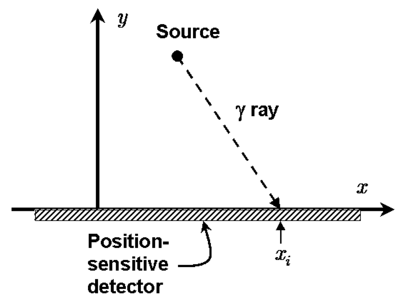
Gamma rays are detected on the $x$ -axis and positions recorded, i.e., $x_{1}, x_{2}, x_{3}, \dots, x_{N} ⟹ {x_{k}}$ .

Goal: Given the recorded positions ${x_{k}}$ , estimate $(x_{0}, y_{0})$ . For the first pass we’ll take $y_{0} = 1$ as known, so we only need to estimate $x_{0}$ (you will generalize later!).

Naively, how would you estimate $x_{0}$ given $x_{1}, \dots, x_{N}$ ? Probably by taking the average of the observed positions. Let’s compare this naive approach to a Bayesian approach.

Follow the notebook leading questions for the Bayesian estimate!

Lecture 2

Contents

1.4. Lecture 2#

Follow-ups to Lecture 1 notebooks#

Bayesian updating via Bayes’ theorem#

Coin tossing example to illustrate updating#

Case I: uniform (flat) prior#

Case II: conjugate prior#

First look at the radioactive lighthouse problem#