Lecture 6

2.3. Lecture 6#

Correlated posteriors#

The pdf for $p(\mu,\sigma|D,I)$ is characterized by elliptical contours of equal probability density whose major axes are aligned with the $\mu$ and $\sigma$ axes. (You can look at the version obtained by sampling in a section appended at the end of this lecture.)
- This is a signal of independent random variables.
- Let’s look at a case where this is not true and then look analytically at what we should expect with correlations.
So return to notebook Parameter estimation example: fitting a straight line
- Review the statistical model.
- What are we trying to find? $p(\thetavec|D,I)$, just as in the other notebooks, now with $\thetavec =[b,m]$.

Comments on the notebook:

Note that $x_i$ is alo randomly distributed uniformly.
Log likelihood gives fluctuating results whose size depend on the # of data points $N$ and the standard deviation of the noise $dy$.

Explore!

Play with the notebook and explore how the size varies with $N$ and $dy$.

Compare priors on the slope $\Longrightarrow$ uniform in $m$ vs. uniform in angle.
Implementation of plots comparing priors:

Questions for the class

With the first set of data with $N=20$ points, does the prior matter?
With the second set of data with $N=3$ points, does the prior matter?

Answers

No!
Yes!

Note: log(posterior) = log(likelihood) + log(prior)
- Maximum is set to 1 for plotting
- Exponentiate: posterior = exp(log(posterior))

What does it mean that the ellipses are slanted?

Answer

It means that the slope and intercept are correlated. Intuitively, if we want to maintain a good fit when we change the slope, we will need to change the intercept as well. They are not independent!

Observations about the second set of data:
- True answers are intercept $b = 25.0$, slope $m=0.5$.
- Flat prior gives $b = -50 \pm 75$, $m = 1.5 \pm 1$, so barely at the $1\sigma$ level.
- Symmetric prior gives $b = 25 \pm 50$, $m = 0.5 \pm 0.75$, so much better.
- Distributions are wide (not surprising since only three points!).

Likelihoods (or posteriors) with two variables with quadratic approximation#

Find $X_0$, $Y_0$ (best estimate) by differentiating

\[\begin{split}\begin{align} L(X,Y) &= \log p(X,Y|\{\text{data}\}, I) \\ \quad&\Longrightarrow\quad \left.\frac{dL}{dX}\right|_{X_0,Y_0} = 0, \ \left.\frac{dL}{dY}\right|_{X_0,Y_0} = 0 \end{align}\end{split}\]

To check reliability, Taylor expand around $L(X_0,Y_0)$:

\[\begin{split}\begin{align} L &= L(X_0,Y_0) + \frac{1}{2}\Bigl[ \left.\frac{\partial^2L}{\partial X^2}\right|_{X_0,Y_0}(X-X_0)^2 + \left.\frac{\partial^2L}{\partial Y^2}\right|_{X_0,Y_0}(Y-Y_0)^2 \\ & \qquad\qquad\qquad + 2 \left.\frac{\partial^2L}{\partial X\partial Y}\right|_{X_0,Y_0}(X-X_0)(Y-Y_0) \Bigr] + \ldots \\ &\equiv L(X_0, Y_0) + \frac{1}{2}Q + \ldots \end{align}\end{split}\]

It makes sense to do this in (symmetric) matrix notation:

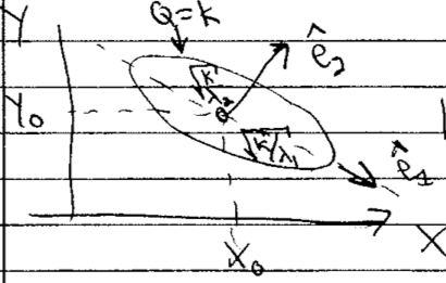
\[\begin{split} Q = \begin{pmatrix} X-X_0 & Y-Y_0 \end{pmatrix} \begin{pmatrix} A & C \\ C & B \end{pmatrix} \begin{pmatrix} X-X_0 \\ Y-Y_0 \end{pmatrix} \end{split}\]

\[ \Longrightarrow A = \left.\frac{\partial^2L}{\partial X^2}\right|_{X_0,Y_0}, \quad B = \left.\frac{\partial^2L}{\partial Y^2}\right|_{X_0,Y_0}, \quad C = \left.\frac{\partial^2L}{\partial X\partial Y}\right|_{X_0,Y_0} \]

So in quadratic approximation, the contour $Q=k$ for some $k$ is an ellipse centered at $X_0, Y_0$. The orientation and eccentricity are determined by $A$, $B$, and $C$.
The principal axes are found from the eigenvectors of the Hessian matrix $\begin{pmatrix} A & C \\ C & B \end{pmatrix}$.

\[\begin{split} \begin{pmatrix} A & C \\ C & B \end{pmatrix} \begin{pmatrix} x \\ y \end{pmatrix} = \lambda \begin{pmatrix} x \\ y \end{pmatrix} \quad\Longrightarrow\quad \lambda_1,\lambda_2 < 0 \ \mbox{so $(x_0,y_0)$ is a maximum} \end{split}\]

What is the ellipse is skewed?

Look at correlation matrix

\[\begin{split} \begin{pmatrix} \sigma_x^2 & \sigma^2_{xy} \\ \sigma^2_{xy} & \sigma_y^2 \end{pmatrix} = - \begin{pmatrix} A & C \\ C & B \end{pmatrix}^{-1} \end{split}\]

Sivia example on “signal on top of background”#

See [SS06] for further details. The figure shows the set up:

The level of the background is $B$, the peak height of the signal above the background is $A$ and there are $\{N_k\}$ counts in the bins $\{x_k\}$. The distribution is

\[ D_k = n_0 [A e^{-(x_k-x_0)^2/2w^2} + B] \]

Goal: Given $\{N_k\}$, find $A$ and $B$.

So what is the posterior we want?

\[ p(A,B | \{N_k\}, I) \ \mbox{with $I=x_0, w$, Gaussian, flat background} \]

The actual counts we get will be integers, and we can expect a Poisson distribution:

\[ p(n|\mu) = \frac{\mu^n e^-\mu}{n!} \ \mbox{$n\geq 0$ integer} \]

or, with $n\rightarrow N_k$, $\mu \rightarrow D_k$,

\[ p(N_k|D_k) = \frac{D_k e^{-D_k}}{N_k!} \]

for the $k^{\text{th}}$ bin at $x_k$.

What do we learn from the plots of the Poisson distribution?

\[\begin{split}\begin{align} p(A,B | \{N_k\}, I) &\propto p(\{N_k\}|A,B,I) \times p(A,B|I) \\ \textit{posterior}\qquad &\propto \quad\textit{likelihood}\quad \times \quad\textit{prior} \end{align}\end{split}\]

which means that

\[ L = \log[p(A,B)|\{N_k\,I\})] = \text{constant} + \sum_{k=1}^M [N_k \log(D_k) - D_k] \]

Choose the constant for convenience; it is independent of $A,B$.
Best point estimate: maximize $L(A,B)$ to find $A_0,B_0$
Look at code for likelihood and prior
Uniform (flat) prior for $0 \leq A \leq A_{\text{max}}$, $0 < B \leq B_{\text{max}}$
- Not sensitive to $A_{\text{max}}$, $B_{\text{max}}$ if larger than support of likelihood

Table of results

Fig. #	data bins	$\Delta x$	$(x_k)_{\text{max}}$	$D_{\text{max}}$
1	15	1	7	100
2	15	1	7	10
3	31	1	15	100
4	7	1	3	100

Comments on figures:

Figure 1: 15 bins and $D_{\text{max}} = 100$
- Contours are at 20% intervals showing height
- Read off best estimates and compare to true
  - does find signal is about half background
- Marginalization of $B$
  - What if we don’t care about $B$? (“nuisance parameter”)
  \[ p(A | \{N_k\}, I) \int_0^\infty p(A,B|\{N_k\},I)\, dB \]
  - compare to $p(A | \{N_k\}, B_{\text{true}}, I)$ $\Longrightarrow$ plotted on graph
- Also can marginalize over $A$
  
  \[ p(B | \{N_k\}, I) \int_0^\infty p(A,B|\{N_k\},I)\, dA \]
- Note how these are done in code: B_marginalized and B_true_fixed, and note the normalization at the end.
Set extra plots to true
- different representations of the same info and contours in the first three. The last one is an attempt at 68%, 95%, 99.7% (but looks wrong).
- note the difference between contours showing the pdf height and showing the integrated volume.
Look at the other figures and draw conclusions.
How should you design your experiments?
- E.g., how should you bin data, how many counts are needed, what $(x_k)_{\text{max}}$, and so on.

Compare Gaussian noise sampling to lighthouse calculation#

Jump to the Bayesian approach in Parameter estimation example: Gaussian noise and averages II and then come back to contrast with the frequentist approach.
The goal is to sample a posterior $p(\thetavec|D,I)$

\[ p(\mu,\sigma | D, I) \leftrightarrow p(x_0,y_0|X,I) \]

where $D$ on the left are the $x$ points and $D$ on the right are the $\{x_k\}$ where flashes hit.
What do we need? From Bayes’ theorem, we need

\[\begin{split}\begin{align} \text{likelihood:}& \quad p(D|\mu,\sigma,I) \leftrightarrow p(D|x_0,y_0,I) \\ \text{prior:}& \quad p(\mu,\sigma|I) \leftrightarrow p(x_0,y_0|I) \end{align}\end{split}\]
You are generalizing the functions for log pdfs and the plotting of posteriors that are in notebook Radioactive lighthouse problem Key.
Note in Parameter estimation example: Gaussian noise and averages I the functions for log-prior and log-likelihood.
- Here $\thetavec = [\mu,\sigma]$ is a vector of parameters; cf. $\thetavec = [x_0,y_0]$.
Step through the set up for emcee.
- It is best to create an environment that will include emcee and corner.
Hint

Nothing in the emcee sampling part needs to change!
- More later on what is happening, but basically we are doing 50 random walks in parallel to explore the posterior. Where the walkers end up will define our samples of $\mu,\sigma$ $\Longrightarrow$ the histogram is an approximation to the (unnormalized) joint posterior.
- Plotting is also the same, once you change labels and mu_true, sigma_true to x0_true, y0_true. (And skip the maxlike part.)
Analysis:
- Maximum likelihood here is the frequentist estimate $\longrightarrow$ this is an optimization problem.
Question

Are $\mu$ and $\sigma$ correlated or uncorrelated?

Answer

They are uncorrelated because the contour ellipses in the joint posterior have their major and minor axes parallel to the $\mu$ and $\sigma$ axes. Note that the fact that they look like circles is just an accident of the ranges chosen for the axes; if you changed the $\sigma$ axis range by a factor of two, the circle would become flattened.
- Read off marginalized estimates for $\mu$ and $\sigma$.