2.1. Lecture 5: Parameter estimation#
Parameter estimation overview comments#
In general terms, “parameter estimation” in physics means obtaining values for parameters (i.e., constants) that appear in a theoretical model that describes data. (Exceptions exist, of course.)
Examples:
couplings in a Hamiltonian
coefficients of a polynomial or exponential model of data
parameters describing a peak in a measured spectrum, such as the peak height and width (e.g., fitting a Lorentzian line shape) and the size of the background
cosmological parameters such as the Hubble constant
Conventionally this process is known as “fitting the parameters” and the goal is to find the “best fit” and maybe error bars.
We will make particular interpretations of these phrases from our Bayesian point of view.
Plan: set up the problem and look at how familiar ideas like “least-squares fitting” show up from a Bayesian perspective.
As we proceed, we’ll make the case that for physics a Bayesian approach is particular well suited.
What can go wrong in a fit?#
As a teaser, let’s ask: what can go wrong in a fit?

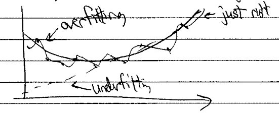
Bayesian methods can identify and prevent both underfitting (model is not complex enough to describe the fit data) or overfitting (model tunes to data fluctuations or terms are underdetermined, leading to them playing off each other).
\(\Longrightarrow\) we’ll see how this plays out.
Notebook: Fitting a line#
Look at Parameter estimation example: fitting a straight line.
Annotations of the notebook:
same imports as before
assume we create data \(y_{\rm exp}\) (“exp” for “experiment”) from an underlying model of the form
\[ y_{\rm exp}(x) = m_{\rm true} x + b_{\rm true} + \mbox{Gaussian noise} \]where
\[ \boldsymbol{\theta}_{\rm true} = [b_{\rm true}, m_{\rm true}] = [\text{intercept, slope}]_{\rm true} \]The Gaussian noise is taken to have mean \(\mu=0\) and standard deviation \(\sigma = dy\) independent of \(x\). This is implemented as
y += dy * rand.randn(N)(noterandn, where the “n” at the end means “normal” distribution).The \(x_i\) points themselves are also chosen randomly according to a uniform distribution \(\Longrightarrow\)
rand.rand(N).Here we are using the
numpyrandom number generators while we will mostly use those fromscipy.statselsewhere.
The theoretical model \(y_{\rm th}\) is:
So in the sense of distributions (i.e., not an algebraic equation),
The last term, which is the model discrepancy (or “theory error”) will be critically important in many applications, but has often been neglected. More on this later!
Here we’ll take \(\delta y_{\rm th}\) to be negligible, which means that
\[ y_i \sim \mathcal{N}(y_{\rm th}(x_i;\boldsymbol{\theta}), dy^2) \]The notation here means that the random variable \(y_i\) is drawn from a normal (i.e., Gaussian) distribution with mean \(y_{\rm th}(x_i;\boldsymbol{\theta})\) (first entry) and variance \(dy^2\) (second entry).
For a long list of other probability distributions, see Appendix A of BDA3, which is what everyone calls Ref. [GCS+13].
We are assuming independence here. Is that a reasonable assumption?
Follow-up on why we called the symmetric prior “the symmetric prior”#
Return to the discussion of priors for fitting a straight line.
Where does \(p(m) \propto 1/(1+m^2)^{3/2}\) come from?
We can consider the prior to be flat in \(m\) and \(b\), or to be flat in the angle between the line and the \(x\)-axis and in the perpendicular distance \(b_\perp=b \cos(\theta)\).
Evaluating the Jacobian for the transformation between \(\theta\) and \(b_\perp\) and \(m\) and \(b\) we find that a flat prior in the former leads to the prior:
\[ p(m,b) = \frac{c}{(1 + m^2)^{3/2}} \]Why is this called “the symmetric prior’‘. Consider the line in which we take \(m'=1/m\) and \(b'=-b/m\). This is the line we would get if we consider the \(x\) as the dependent variable and \(y\) as the independent variable: \(x=y/m - b/m\). If we require that the problem be invariant under interchange of the \(x\) and \(y\) axes then we should rqeuire that the prior on \(m,b\) (i.e., \(p(m,b)\)) has the same functional form as those on \(m',b'\) (so \(p(m',b')\) with the same function \(p\)). This argument is due to Jaynes (1973), although Gull (1989) disagrees with Jaynes’ argument.
Then for the probabilities, we must have
Evaluating the Jacobian gives \(1/m^3\), so we need to solve the functional equation:
Which our prior obeys.
Check that the prior satisfies (2.1)
Answer
\[ p(1/m, -b/m) = \frac{c}{(1 + (1/m)^2)^{3/2}} = \frac{c}{\frac{1}{m^3}(m^2 + 1)^{3/2}} = m^3 p(m,b) \quad \]It works! Note that this prior is independent of \(b\).
