3.1. Lecture 7#
Why MCMC?#
This discussion is based heavily on Gregory [Gre05], Chapter 12.
We have been emphasizing that in the Bayesian approach, everything is a pdf. One type of pdf is for the parameters of a theory, which we’ll denote by the vector \(\thetavec\), given data \(D\) and information \(I\), namely \(p(\thetavec|D,I)\). Suppose we have a theoretical model for this.
Examples
Parameters determining a density functional.
Low-energy constants for an effective field theory Hamiltonian.
And now we want to calculate the expectation value of a function of \(\thetavec\), e.g., \(\langle f(\thetavec)\rangle\).
Another example would be if \(\thetavec\) characterized a signal and background and we had a function of the signal.
As we discussed in doing the central limit theorem:
This is more involved than what is done in conventional calculations, in which we would have single values of \(\thetavec\), maybe denoted \(\widehat{\thetavec}\), that we might have found by minimizing a \(\chi^2\) function.
E.g., we identified the particular values of \(\theta_1, \theta_2,\ldots\theta_n\) that specify a nuclear force Hamiltonian that best reproduced neutron-proton scattering data. Then we would want to calculate \(\langle f(\thetavec)\rangle\), which might be the binding energy of a nucleus (a very complicated function in this case!).
But \(\langle f(\thetavec)\rangle\) means we must do a multidimensional integral over the full range of possible \(\thetavec\) values, weighted by the probability density function \(p(\thetavec|D,I)\), which we have worked out already.
This is a lot more work!
We frequently also have a situation where we want to integrate (marginalize) over a subset of parameters \(\thetavec_B\) to find a posterior for the rest \(\thetavec_A\). E.g., over parameters for the width of a signal and other parameters characterizing our model for the Higgs mass.
These multidimensional integrals then become a necessity to do, but conventional methods for low dimension (e.g, Gaussian quadrature of Simpson’s rule) become inadequate rapidly with the increase of dimension.
The integrals in question are particularly problematic because the posteriors are very small in much of the integration volume, which will typically also be a challenging shape.
To approximate such integrals one turns to Monte Carlo (MC) methods. The straight (naive) MC integration evaluates the integral by randomly distributing \(n\) points in the multidimensional volume \(V\) of possible \(\thetavec\)’s. \(V\) has to be large enough to cover where \(p(\thetavec|D,I)\) is significantly different from zero.
Then we have
where
Caution
\(\thetavec_i\) is the \(i^{\text{th}}\) set of \(\thetavec\) values, not a component of \(\thetavec\).
More details on naive MC
In one dimension, the average of a function
from calculus. But we can estimate \(\overline g(\theta)\) by averaging over a set \(n\) of random samples \(\{\theta_i\}\):
Then the expectation value of \(f(\theta)\) is
Here \(b-a\) is the “volume” \(V\) in one dimension.
Does this always work? No! (Cf., the radioactive lighthouse problem.) But if the central limit theorem applies, it should work, but maybe not efficiently.
The uncertainty is assuming that a Gaussian approximation is valid. Note the dependence on \(1/\sqrt{n}\), which means you can get a more precise answer by increasing \(n\). But slowly better; each additional decimal point accuracy costs you a factor of 100 in \(n\).
Markov Chain Monte Carlo (MCMC)#
Key problem: too much time is wasted sampling regions where \(p(\thetavec|D,I)\) is very small. If for one parameter the fraction of significant strength is \(10^{-1}\), in an \(M\)-parameter problem the fraction of the volume is \(10^{-M}\). This necessitates importance sampling, which reweights the integrand to more appropriately distribution points (e.g., the program VEGAS), but this is difficult to accomplish in general.
Bottom line: it is not feasible to draw a series of independent random samples from \(p(\thetavec|D,I)\) for larger sizes of \(\thetavec\).
Remember, independent means if \(\thetavec_1, \thetavec_2, \ldots\) is the series, knowing \(\thetavec_i\) doesn’t tell us anything about \(\thetavec_{i+1}\) (or any other \(\thetavec\)).
But the samples don’t need to be independent. We just need to generate \(p(\thetavec|D,I)\) in the correct proportions (e.g., so it approximates \(p(\thetavec|D,I)\) when histogramming the samples).
Solution: Do a random walk (diffusion) in the parameter space of \(\thetavec\), so that the probability for being in a region is proportional to \(p(\thetavec|D,I)\) for that region.
\(\thetavec_{i+1}\) follows from \(\thetavec_i\) by a transition probability (“kernel”) \(\Lra\) \(p(\thetavec_{i+1}|\thetavec_i)\).
The transition probability is assumed to be “time independent”, so same \(p(\thetavec_{i+1}|\thetavec_i)\) no matter when you do it \(\Lra\) Markov chain and the method is called Markov Chain Monte Carlo or MCMC.
Once we have a representative set of \(N\) vectors \(\{\thetavec_i\}\), then any expectation value of a function \(f\) of \(\thetavec\), which is the integral of \(f(\thetavec) p(\thetavec|D,I)\) over \(\thetavec\), is given simply by the average \(\langle f\rangle = \frac{1}{N}\sum_i f(\thetavec_i)\).
We can think of the sampled distribution as a set of delta functions, whose normalization is trivial:
Check that with the delta functions we get the rule for \(\langle f\rangle\).
Basic structure of MCMC algorithm#
Given \(\thetavec_i\), propose a value for \(\thetavec_{i+1}\), call it the “candidate” \(\phivec\), sampled from \(q(\phivec|\thetavec_i)\). This \(q\) could take many forms, so for concreteness imagine it as a multivariate normal distribution with mean given by \(\thetavec_i\) and variance \(\sigmavec^2\) (to be specified).
Decreased probability as you get further away from the current sample.
\(\sigmavec\) determines the step size.
Decide whether or not to accept candidate \(\phivec\) for \(\thetavec_{i+1}\). Here we’ll use the Metropolis condition (later we’ll see other ways that may be better).
This dates from the 1950’s in physics but didn’t become widespread in statistics until almost 1980.
Enabled Bayesian methods to be much more widely applied.
Metropolis condition
Calculate Metropolis ratio \(r\) given current \(\thetavec_i\) and proposed candidate \(\phivec\):
The distribution \(q\) may be symmetric: \(q(\thetavec_1|\thetavec_2) = q(\thetavec_2|\thetavec_1)\). If so, then this is called “Metropolis”. If not, then it is called “Metropolis-Hastings”.
Decision:
If \(r\geq 1\), set \(\thetavec_{i+1} = \phivec\) \(\Lra\) always accept
If \(r < 1\), so less probable, don’t always reject! Accept with probability \(r\) by sampling a Uniform (0,1) distribution. (Because \(0\leq r\leq 1\) for this case we can take \(r\) as a probability.)
In practice we carry out the \(r<1\) case by getting a sample \(U \sim \text{Uniform}(0,1)\). If \(U \leq r\), then \(\thetavec_{i+1} = \phivec\), else \(\thetavec_{i+1} = \thetavec_i\).
Note that the last case means you do have a \(\theta_{i+1}\), but it is the same as \(\theta_i\) (so you have multiple copies and the chain continues to grow).
The acceptance probability is the minimum of \(1,r\).
Algorithm pseudo-code:
Initialize \(\thetavec_i\), set \(i=0\).
Repeat
{
Obtain new candidate \(\phivec\) from \(q(\phivec|\theta_i)\) Calculate \(r\) Sample \(U \sim \text{uniform}(0,1)\) If \(U \leq r\) set \(\thetavec_{i+1} = \phivec\), else set \(\thetavec_{i+1} = \thetavec_i\).
\(i++\)
}
It’s important to do the else step for \(U \gt r\).
Plan:
Look at visualizations.
Look at a basic example for the Poisson distribution.
Consider MCMC_random_walk_and_sampling notebook.
Look at
emceeexample from Assignment 1.
Visualization of MCMC sampling#
There are excellent javascript visualizations of MCMC sampling out there.
A particularly effective set of interactive demos was created by Chi Feng, available at https://chi-feng.github.io/mcmc-demo/
These demos range from random walk Metropolis-Hastings (MH) to Adaptive MH to Hamiltonian Monte Carlo (HMC) to No-U-Turn Sampler (NUTS) to Metropolis-adjusted Langevin Algorithm (MALA) to Hesian-HMC (H2MC), to Stein Variational Gradient Descent (SVGD) to Nested Samplig with RadFriends (RadFriends-NS).
An accessible introduction to MCMC with simplified versions of Feng’s visualization by Richard McElreath. Let’s look at the first part of his blog entry at http://elevanth.org/blog/2017/11/28/build-a-better-markov-chain/.
Recall the basic structure of Metropolis-Hastings
Make a random proposal for new parameter values.
Accept or reject the proposal based on a Metropolis criterion.
Random Walk Metropolis-Hasting (MH)#
Here are some comments and observations on the basic MH simulation.
The target distribution is a two-dimensional Gaussian (just the product of two one-dimensional Gaussians).
Question
Is the distribution correlated? How do you know?
An uncolored arrow indicates a proposal, which is accepted (green) or rejected (red).
Notice that the direction and the length of the proposal arrow varies and are, in fact, chosen randomly from a distribution. The direction is sampled uniformly.
The MH MCMC seems to do ok on sampling such a simple distribution, as indicated by how well the projected posteriors get filled in.
But it is diffusing, i.e., a random walk, which is not so efficient. A more complicated shape can cause problems:
MH can spend a lot of time exploring over and over again the same regions;
if not specially tuned, many proposals can be rejected (red arrows).
The donut shape is much trickier
Notice that the projected one-dimensional posteriors don’t seem to be so complex, but this is a difficult topology.
Is it realistic? The claim is that when there are many parameters (a high-dimensional space), this is analogous to a common target distribution.
Problems: we are constantly looking for the right step size, which is big enough to explore the space, but small enough to not get rejected too often.
High dimensions is a big space! It is hard to stay in a region of high probability while also exploring enough (in a reasonable time).
Note on donuts in high dimensions

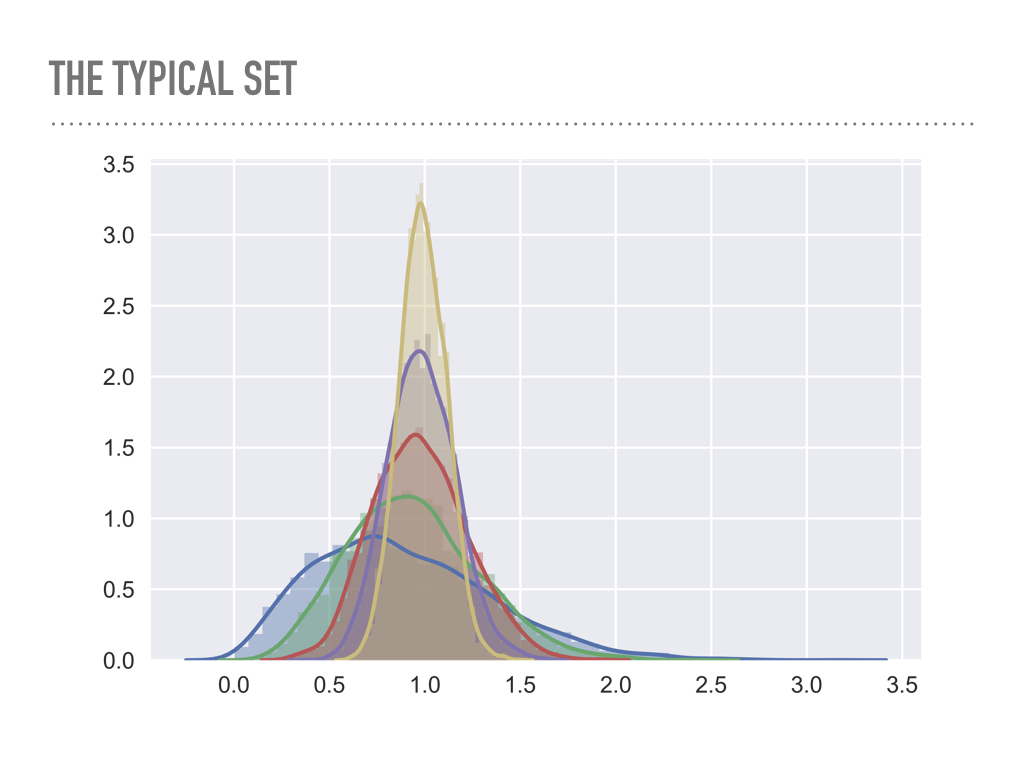
Look at the average radius of points sampled from multivariate Gaussians as a function of the dimension.
blue is one dimensional, green is two dimensional, … , yellow is six dimensional.
Imagine yellow as a 6-dimensional shell \(\Lra\) analog is a two-dimensional donut.
Take a look at the Feng site.
The banana distribution \(\Lra\) difficult to sample.
If multimodal \(\Lra\) very, very tough.
Try adjusting the proposal \(\sigma\) (Gaussian proposal with variance \(\sigma^2\)) \(\Lra\) try this on donut: to get green you need excellent step size tuning.
Back to the McElreath page. What is the answer to better sampling? His claim: “Better living through physics”
This means to use Hamiltonian Monte Carlo (HMC).
Later we’ll come back to HMC but stick with MH for now.
Metropolis Poisson example (Gregory, section 12.2)#
See Metropolis-Hasting MCMC sampling of a Poisson distribution.
We’ve already seen the Poisson distribution \(p(k|\mu) = \mu^k e^{-\mu}/k!\) for integer \(k\geq 0\) and we’ve sampled it through a
scipy.statsscript. Here we’ll sample it via MCMC.Basic Markov chain: starts with some initial value, then each successive one is generated from the previous.
Step through the procedure for Poisson, then step through the code.
Look at the two graphs produced.
MCMC trace: value at successive MC steps. Notice the fluctuations; it stays reasonably close to 3 (the value of \(\mu\)) but still can jump high.
The histogram shows how well we’ve doing.
Use
cntl-enterto run many times.Note the outliers at the beginning: the sampling needs to equilibrate. This is called the warm-up (or “burn-in”) time.
How do you expect the trace to behave for different \(\mu\)?
Do the questions.
Note: the proposal pdf is asymmetric
symmetric means that the probability to jump to \(\thetavec_{\text{now}}\) from \(\thetavec^t\) is the same as the likelihood of jumping back to \(\thetavec^t\) from \(\thetavec_{\text{now}}\).
Typically \(\mathcal{N}(\thetavec^t,\sigmavec)\) with fixed \(\sigmavec\).
Symmetric because difference of \(\thetavec^t, \thetavec_{\text{now}}\) appears squared.
